Bayesian Deep Learning

This sentense sums up what we're trying to achieve through data science and here bayesian data analysis : implement models who can adapt to the data you feed it on input, no matter its size as long as it is consistent with the nature of the data the model has been trained with.

When we think about time series forecasting, it is common to use Neural Network in order to forecast our predictions by using either ANN or LSTM/GRU RNNs in order to make single-step or multi-step forecasting.
Yet, even though time series forecasting gives pretty good results with common deep learning approaches, it is still important to quantify the uncertainty on te predictions made by such models. This is why we're gonna implement a neural network with a quantification of the prediction uncertainty : a Bayesian neural network.

The theory on this topic shall be exposed in another article, the main thing to keep in mind is that the Bayesian neural network implemented here is based on a principle called : Variational Inference.
Basically, the intuition behind this concept is we're trying to approach the true posterior distribution \(p(y|x)\) with an approximation \(q(x)\)

The model will be implemented with Tensorflow Probability. It is a new framework designed to incorporate probabilistic programming in machine learning and deep learning models. Here we'll implement a bayesian neural network.

The project will consist in 2 parts :

1. Regression with Tensorflow probability on artificial data
2. Application of variational inference on real world data : stock forecasting

To begin this project, we'll need to precise 2 variables we'll instanciate for the rest of the project besides all the necessary known packages of Pandas and NumPy :

import tensorflow_probability as tfp
								
tfd = tfp.distributions

Let's create our artificial data :

w0 = 0.125
b0 = 5.
x_range = [-20,60]
							
def load_dataset(n=150, n_tst=150):
  np.random.seed(42)
  def s(x):
    g = (x - x_range[0]) / (x_range[1] - x_range[0])
    return 3 * (0.25 + g**2.)
							
  x = (x_range[1] - x_range[0]) * np.random.randn(n) + x_range[0]
  eps = np.random.randn(n) * s(x)
  y = (w0 * x * (1. + np.sin(x)) + b0) + eps
  x = x[...,np.newaxis]
  x_tst = np.linspace(*x_range, num=n_tst).astype(np.float32)
  x_tst = x_tst[...,np.newaxis]
  return y, x, x_tst
							
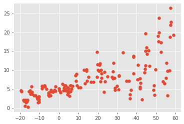
y, x, x_tst = load_dataset()
							
plt.figure()
plt.scatter(x,y)
plt.show()

We get the following dataset :

In order to approximate the distribution of this dataset, we'll create a neural network with a dense layer and add a distribution to the layer with DistributionLambda method implemented in Tensorflow Probability.

noise = 1.0
def neg_log_likelihood(y_true, y_pred, sigma=noise):
  dist= tfd.Normal(loc=y_pred, scale=sigma)
  return tf.reduce_sum(-dist.log_prob(y_true)) 
							
model = tf.keras.layers.Sequential([
                      tf.keras.layers.Dense(1 + 1),
                      tfp.layers.DistributionLambda(lambda t: tfd.Normal(loc=t[...,1], scale=1e-3 + tf.math.softplus(0.05 * t[...,1:])))
])
							
model.compile(optimizer= tf.optimizer.Adam(learning_rate= 0.01), loss=neg_log_likelihood)
model.fit(x, y, epochs=1000, verbose=False)
							
[print(np.squeeze(w.numpy())) for w in model.weights]
y_hat = model(x_tst)
							
plt.figure(figsize=(7,5))
plt.plot(x, y, 'b.', label="observed")
							
m = y_hat.mean()
s = y_hat.stddev()
							
plt.plot(x_tst, m, "r"), lw=2, label=mean prediction)
plt.plot(x_tst, m + 2 * s, 'g', lw=2, label="mean + 2 * std")
plt.plot(x_tst, m - 2 * s, 'g', lw=2, label="mean - 2 * std")
							
plt.ylim(0.,17)
plt.yticks(np.linspace(0,15, 4)[1:])
plt.xticks(np.linspace(*x_range, 9))
plt.legend()
							
plt.show()

What we did here :
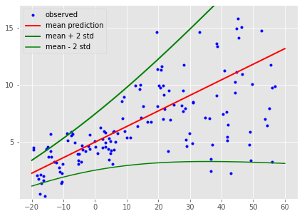
1. We created a neural network architecture with Tensorflow with : tf.keras.layers.Sequential()
2. We added a probabilistic distribution to a Dense layer with tfp.layers.DistributionLambda()
3. We've set up our probabilistic distribution to be a Normal distribution
4. The standard deviation of our Normal distribution is parametrized by a softplus function in order to keep the variance positive

The mecanism which make possible to update weights through a bayesian neural network is called a "reparametrization trick", we'll discuss about this topic later on the theoretical part of the project.

Tensorflow uses a method DenseReparametrization to make the mecanism of probabilistic weight distribution update possible combined with DenseFlipout to have a full "bayesian" layer.
Since the Tensorflow 2.0 release, there seem to be a few issues with the methods which is why the tensorflow team recommends to use DenseVariational method which give a result similar to the combination of the 2 others but without the Flipout.

Application to real world application : GOOG stock prediction

We'll now apply our probabilistic framework to a real-world case to do some time series forecast. We won't care about stationarizing our time series neither about the level, seasonality nor other feature to see how a simple Bayesian Neural network manages to predict on a walk-forward process the behavior of our time series.

let's import our data and see what we have there:

df_goog = pd.read_csv(r"GOOG.csv")
df_goog.head()

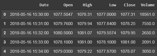
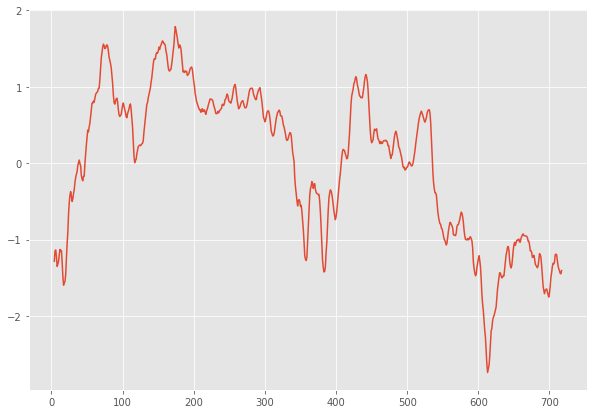
When we deal with time series, it is often the case that we have some noise in our signal when the frequency of the signal is very important just like for our GOOG stock :

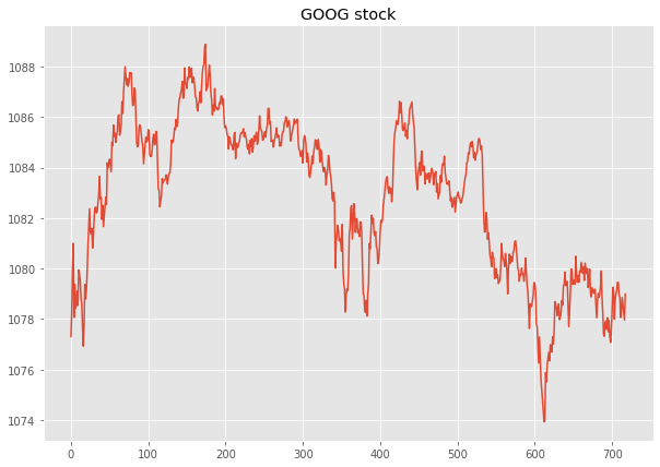
According to how noisy our signal can be, we can apply more-or-less filtering on it in order to have more accurate estimations from our models. We have 1-minute dataset for open-high-low-close, on GOOG stock which we'll smooth with a moving average every 5 mins in order lower the data noise at the very minimum for our prediction.

df_goog_standardized = (df_goog['Close'] - df_goog['Close'].mean())/df_goog['Close'].std()
								
plt.figure()
df_goog_standardized.rolling(5).mean().plot(figsize=(10,7))

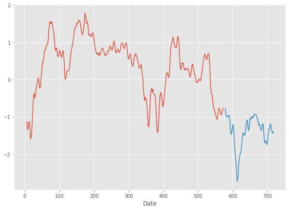
Let's do our train-test split on this dataset then :

We build our model using mean shift variational inference model in order to approximate our true posterior, to have some intuition, approximating the true posterior distribution can be a pain and not give very good results, a method called mean shift variational inference (which will be explained more in detail in another article) is up until today, the best one to estimate this distribution \(q(x)\) where we make the assumption that the distribution will be of the form \(Q_{MFVB} := \{ q : q(\theta) = \prod_{j=1}^{J}q_j(\theta_j)\} \) with \(\theta\) our parameter vector, we assume that our approximate distribution factorizes over each of our components \(\theta_1,...,\theta_J \). For us it is very simple, our parameters are the mean and the variance of our prior distribution:

def posterior_mean_field(kernel_size, bias_size=0, dtype=None):
  n = kernel_size + bias_size
  c = np.log(np.expm1(1.))
  return tf.keras.Sequential([
                   tfp.layers.VariableLayer(2 * n, dtype=dtype),
                   tfp.layers.DistributionLambda(lambda t:tfd.Independent(tfd.Normal(loc=t[...,:n], scale=1e-5 + tf.nn.softplus(c + t[...,n:])), reinterpreted_batch_ndims=1))
  ])
								
def prior_trainable(kernel_size, bias_size=0, dtype=None):
  n = kernel_size + bias_size
  return tf.keras.Sequential([
                   tfp.layers.VariableLayer(n, dtype=dtype),
                   tfp.layers.DistributionLambda(lambda t:tfd.Independent(tfd.Normal(loc=t, scale=1), reinterpreted_batch_ndims=1))
  ])
								
model = tf.keras.Sequential([
                 tfp.layers.DenseVariational(24, posterior_mean_field, prior_trainable, kl_weight=1/x_train.values.shape[0], activation='relu'),
                 tfp.layers.DenseVariational(1, posterior_mean_field, prior_trainable, kl_weight=1/x_train.values.shape[0])
])
								
model.compile(optimizer= tf.optimizers.Adam(learning_rate=0.01, loss=neg_log_likelihood))
model.fit(x_train, y_train, epochs=250)

Once fit, we'll plot the result of prediction with the uncertainty of the model on the results.

plt.figure(figsize=(10,7))
plt.clf()
								
nans = np.empty(len(y_train))
nans[:] = np.nan
y_test_plot= np.r_[nans, y_test.values]
								
plt.plot(y_train)
plt.plot(y_test_plot, 'b', label='observed')
								
y_hats_list = [model(x_test.values.reshape(-1,1)).numpy() for _ in tqdm(range(50))]
y_hats = np.concatenate(y_hats_list, axis=1)
								
m, s1, s2 = np.mean(y_hats, axis=1), np.percentile(y_hats, 5, axis=1), np.percentile(y_hats, 95, axis=1)
m_plot, s1_plot, s2_plot = np.r_[nans, m], np.r_[nans, s1], np.r_[nans, s2]
								
plt.plot(m_plot, 'g', label="ensemble mean")
plt.fill_between(np.linspace(1, len(m_plot), len(m_plot)), y1=s1_plot, y2=s2_plot, alpha=0.4, color="grey", label="prediction interval")
								
plt.legend(loc=3)
plt.show()

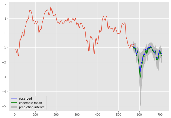
Let's look at a closer look to predict our test set.

these results are pretty encouraging for the prediction of our stock data with a Negative Likelihood of ~29. This is a simple demonstration of how simple we can now build a bayesian neural network to make a prediction and to quantify the uncertainty on the forecast of our model.