Bayesian time series forecasting : Random Walk & applications (part 2)

This part is the 2nd part of the bayesian time series prediction articles, in this one we'll discuss on random walk, bayesian method and application to time series forecasting.

For this part, we'll not talk about theory on random walk in which I'll talk about in an article in another section of the website. To keep it straight, we'll just use the necessary hypothesis and formulations to show how this small project was implemented. Let's get started !

The time series used in the last article had a very useful property called "Stationarity" which made us able to use econometric models. For this part, we'll work on real life example to predict the trend of a stock. But in financial world and in every area within a complex environment where statistics are used, it's important to keep in mind that every implemented model will potentially not work any longer after a while, not because of a disfunction or a bug in your code, but because the context is simply no longer the same.

In general, we won't have the chance to have stationary time series and it happens a lot of time we can't just stationarize them. So here we decide to make the assumption that the time series we'll fit with our model are non-stationary and we won't try to change it.

This is why what is working here don't have any pretention of being a production ready model. Yet the obtained results are interesting for several time series datasets and I will publish more developped model later on a next article.

For now, we'll work on 2 stock data :

1. GOOG stock
2. ETH/USD stock

df_goog = pd.read_csv("../goog_stock.csv")
							
...(data preprocessing)...
							
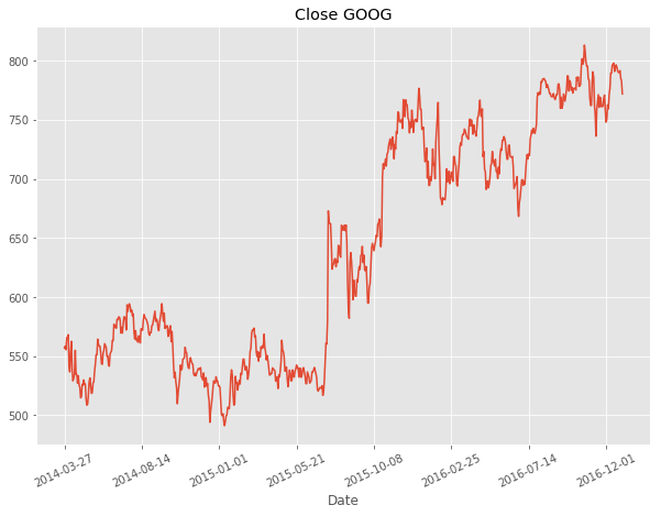
df_goog.set_index("Date")["Close"].plot(figsize(10,7), title="Close GOOG")
plt.xticks(rotation=25)

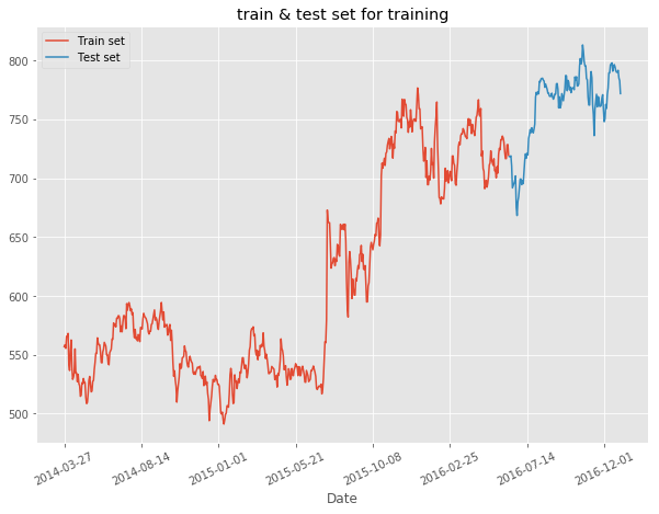
We then split our dataset in train & test sets where we take the first 80% of our time series for train set and the rest for the test set.

train = df_goog['Close'][:int(len(df_goog)*0.8)]
test = df_goog['Close'][int(len(df_goog)*0.8):]
plt.figure(figsize=(10,7))
plt.plot(train, label="Train set")
plt.plot(test, label="Test set")
plt.xticks(df_goog.index[::100],rotation=25)
plt.xlabel("Date")
plt.title("train & test set for training")
plt.legend()
plt.show()

In order to build our bayesian model, we're gonna use a python framework named PyMC3 which is the reference library for bayesian model implementation. It is based on Theano which is an open source deep learning framework. We'll use it to put our variables in tensors with shared which will be very useful to change the observation variable in our bayesian model.

observed_shared = shared(train.values)
train_shared = shared(train.shape[0])
test_shared = shared(test.shape[0])

From there, we'll build our model named ts_model_goog

ts_model_goog = pm.Model()
with ts_model_goog:
  sd = pm.HalfNormal('sd', sd=.5)
  mu = pm.Normal('mu', mu=0, sigma=1.)
  z = pm.GaussianRandomWalk("z",mu=mu, sd=sd, observed=observed_shared)
  trace = pm.sample(2000)

This model is a sampling algorithm based on a principle called MCMC - Markov Chain Monte Carlo which is a mix of a graph and a sampling method. We build a graph of the values of the distribution and each of the node of the graph is linked to the next most probable value to be sampled. Every node of the chain are only depending on the previous node. Such a graph is generated randomly through the Monte-Carlo sampling method.

Then, we'll sample from the posterior predictive distribution after replacing the shape of the observation with the test set shape in order to have a sampling of the right size. To change the value of the observation we'll use a theano tensor method : [theano_tensor].set_value(..)

test_observed = np.empty((test.shape[0],))
observed_shared.set_value(test_observed)

From here we sample to have our prediction :

with ts_model_goog:
  ppc_test = pm.sample_posterior_predictive(trace,samples=2000)

Then, let's plot our prediction :

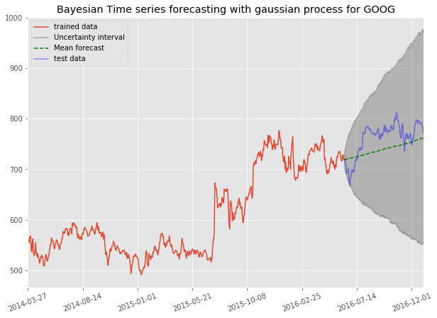
Indeed, we can see the uncertainty area is huge and the error of our mean prediction with the real values is quite important, nevertheless the model seem to capture the trend of the GOOG stock quite well without any information but the time series. It would be interesting to see how to include some more information in order to have a more accurate prediction and keep a good quantification of the uncertainty.

If we just plotted the mean prediction with the standard deviation from the mean, we would have gotten some very unaccurate uncertainty quantification. Here we can intuitively and physically admit that for any stock the uncertainty is great when we don't have any other parameter. Yet as we would have deduced ourself, the trend of such a stock is clearly upward and it gives us a frame in which we could consider our prediction for this stock.

So what use of such a model where we could have deduced the conclusion ourself ? Well as we said, models can work well but potentially could fail as well. The point of this implementation is to show we can build simple model to be used as an indicator to take some decision and not to replace our jugement. Of course here we started at a very basic level but in further articles we'll produce more complex models but on a solid basis.

In a next article, I'll go deeper into the theory of how this model is working and the background necessary to understand the mecanics of it.